Statistical analysis involves a sequence of mathematical computations for comparing treatments and evaluating whether any observed differences are truly a result of the change in practices, or if the differences may be due to chance and natural variation.
This section looks at statistical analysis in more detail, expanding on step 9 in the process outlined earlier. Recall that the type of statistics you use to analyze your data follows directly from your experimental design (Table 2). The two types of statistical analysis covered here are the t-test and ANOVA. You can learn to do your own data analysis either by hand or using a statistical software program. In most situations, you will also want to consult with your agricultural advisor or Cooperative Extension personnel for guidance and assistance with your data analysis. Before we get into the specifics of those techniques, here is a review of some basic statistics terminology:
Normal distribution: The normal distribution describes a collection of data organized around an average value (the mean), with greater or lesser data points distributed approximately equally on either side of that value. The data in a normal distribution is often described as following a bell-shaped curve (Figure 7). This phenomenon occurs regularly in nature and is the basis for the statistics we use in on-farm research. Using an agricultural example, if you recorded the average corn yield from all the farmers in a given area, those yields would probably follow a normal distribution. The key features of the normal distribution are the mean, or average value, and the variance, or how widely the data is spread around the mean.
Mean: The mean is the average value in a data set. You calculate the mean by adding up all the data points in the group and then dividing the total by the number of data points.
Variance: The variance in a collection of data describes the extent to which the high and low values differ from the mean value. Figure 7b shows three normal distribution curves with different variances.
Standard deviation: The standard deviation, which is the square root of the variance, is more typically used to analyze how your data varies from the mean. A small standard deviation means that the data is clustered closely around the mean; a large standard deviation means the data is spread out over a wider range of values. The standard deviation is expressed in the same units as the data (e.g., bushels per acre).
Standard error: This term usually refers to the “standard error of the mean.” In statistical analysis you often want to know how representative a certain sample size is of the overall population. When you collect samples and calculate a mean, this data presents a snapshot of the system you are studying but it is not an exact representation because there is data that you did not collect. If you were to repeat your sampling procedure, or collect more or fewer samples, you would get somewhat different data with a different mean. So, calculating standard error is a way of estimating how representative your data actually is of the population within the system you are studying. The standard error is basically calculated as the standard deviation of the distribution of sample means taken from a population. The smaller the standard error, the more representative that sample is of the overall population. Also, as the number of samples you take to make the standard error calculation increases, the standard error decreases.
Error: In the analysis of research data, you may still come to the wrong conclusion. There are two kinds of errors in statistical analysis: a Type I error and a Type II error. A Type I error occurs when you identify a difference when in fact the treatments were not different. A Type II error is the opposite, when you determine there is no difference yet in fact there really is. A probability level, typically 5 percent in field research, is used to indicate the likelihood that a Type I or Type II error will occur. This concept is closely related to the concept of statistical significance, described next.
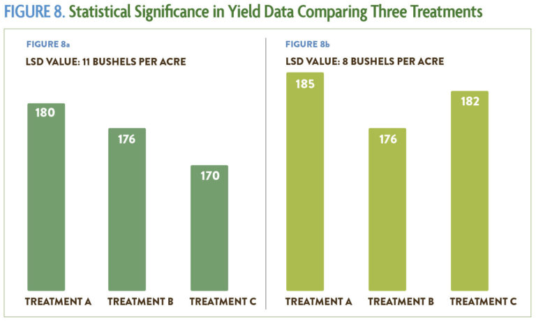
Statistical significance/Least significant difference: In statistics, significance of results does not refer to how important those results are. Rather, a statistically significant finding means that the researcher is confident that the result is reliable within certain parameters. In other words, the treatment had an actual effect on the system, and the results were not the product of chance. This concept is captured by a numerical value known as the least significant difference (LSD). Any difference between treatment practices that is greater than the LSD value means the difference you identified is most probably a result of the treatment, whereas a smaller difference is likely to be the result of chance—you cannot guarantee the same results if you repeated the experiment. The least significant difference is always noted at a certain confidence level, usually 90 or 95 percent, which tells you the probability that a Type I error could occur. For example, a 90 percent confidence level means there is still a 10 percent chance the difference was actually due to natural variation. Sometimes you will see the confidence level identified by its corresponding alpha value: A 95 percent confidence level has an alpha of 5 percent (LSD 0.05) and a 90 percent confidence level has an alpha of 10 percent (LSD 0.1). Anything less than 90 percent certainty is usually not considered scientifically valid. This concept is crucial to understanding and interpreting your results, so more information is provided in the calculations that follow.
Sum of squares: This is a measure of variation or deviation from the mean (average). It is calculated by finding the difference between each individual data point and the mean of all the data points, then squaring each difference and adding all the squared values.


